recurrent networks

Recurrent Neural Networks (RNNs) are popular models that have shown great promise in many NLP tasks. But despite their recent popularity I’ve only found a limited number of resources that throughly explain how RNNs work, and how to implement them. That’s what this tutorial is about. It’s a multi-part series in which I’m planning to cover the following:

1. Introduction to RNNs (this post)
2. Implementing a RNN using Python and Theano
3. Understanding the Backpropagation Through Time (BPTT) algorithm and the vanishing gradient problem
4. Implementing a GRU/LSTM RNN

As part of the tutorial we will implement a recurrent neural network based language model. The applications of language models are two-fold: First, it allows us to score arbitrary sentences based on how likely they are to occur in the real world. This gives us a measure of grammatical and semantic correctness. Such models are typically used as part of Machine Translation systems. Secondly, a language model allows us to generate new text (I think that’s the much cooler application). Training a language model on Shakespeare allows us to generate Shakespeare-like text. 

I’m assuming that you are somewhat familiar with basic Neural Networks. If you’re not, you may want to head over to Implementing A Neural Network From Scratch,  which guides you through the ideas and implementation behind non-recurrent networks.

WHAT ARE RNNS?

The idea behind RNNs is to make use of sequential information. In a traditional neural network we assume that all inputs (and outputs) are independent of each other. But for many tasks that’s a very bad idea. If you want to predict the next word in a sentence you better know which words came before it. RNNs are called recurrent because they perform the same task for every element of a sequence, with the output being depended on the previous computations. Another way to think about RNNs is that they have a “memory” which captures information about what has been calculated so far. In theory RNNs can make use of information in arbitrarily long sequences, but in practice they are limited to looking back only a few steps (more on this later). Here is what a typical RNN looks like:

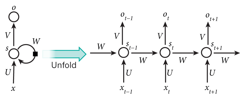
A recurrent neural network and the unfolding in time of the computation involved in its forward computation. Source: Nature

The above diagram shows a RNN being unrolled (or unfolded) into a full network. By unrolling we simply mean that we write out the network for the complete sequence. For example, if the sequence we care about is a sentence of 5 words, the network would be unrolled into a 5-layer neural network, one layer for each word. The formulas that govern the computation happening in a RNN are as follows:

•  is the input at time step . For example,  could be a one-hot vector corresponding to the second word of a sentence.
•  is the hidden state at time step . It’s the “memory” of the network.  is calculated based on the previous hidden state and the input at the current step: . The function  usually is a nonlinearity such astanh or ReLU.  , which is required to calculate the first hidden state, is typically initialized to all zeroes.
•  is the output at step . For example, if we wanted to predict the next word in a sentence it would be a vector of probabilities across our vocabulary. .

There are a few things to note here:

• You can think of the hidden state  as the memory of the network. captures information about what happened in all the previous time steps. The output at step  is calculated solely based on the memory at time . As briefly mentioned above, it’s a bit more complicated  in practice because typically can’t capture information from too many time steps ago.
• Unlike a traditional deep neural network, which uses different parameters at each layer, a RNN shares the same parameters ( above) across all steps. This reflects the fact that we are performing the same task at each step, just with different inputs. This greatly reduces the total number of parameters we need to learn.
• The above diagram has outputs at each time step, but depending on the task this may not be necessary. For example, when predicting the sentiment of a sentence we may only care about the final output, not the sentiment after each word. Similarly, we may not need inputs at each time step. The main feature of an RNN is its hidden state, which captures some information about a sequence.

WHAT CAN RNNS DO?

RNNs have shown great success in many NLP tasks. At this point I should mention that the most commonly used type of RNNs are LSTMs, which are much better at capturing long-term dependencies than vanilla RNNs are. But don’t worry, LSTMs are essentially the same thing as the RNN we will develop in this tutorial, they just have a different way of computing the hidden state. We’ll cover LSTMs in more detail in a later post. Here are some example applications of RNNs in NLP (by non means an exhaustive list).